How to Read a Vapor Liquid Equilibrium Diagram

Explanation:

A pure component, like water for example, can exist in multiple phases: as a solid, liquid, or a vapor/gas. Say, we put a pan of water in the freezer where information technology freezes the h2o in it. If we take it out, place it on a burner, and plough on oestrus, we volition eventually melt the ice. The temperature throughout the melting is constant, and for water, it is its melting point of 0°C. That is, from the moment that the commencement drop of liquid forms until the bespeak at which we have near completely melted the ice, information technology is at 0°C. Afterwards it is all liquid, we can simply add heat to the system until the temperature of the solution reaches 100°C, where the temperature once again stays constant until the liquid is completely vaporized. If we trapped the vapor after it is formed, we could keep to heat information technology to raise its temperatures far above 100°C. Note, for this process, the pressure was held abiding; we were at constant atmospheric pressure level.

The post-obit phase diagram is representative of water. The path just discussed is the red path A on the diagram. That is, taking ice from sub-cooled temperatures (say, in the freezer it was -8°C) is to left of the orange line. We raise the temperature to its melting point where the temperature is constant (from the point the showtime drib forms to the point were the terminal chip of ice melts) is the temperture right on the orange line. Between the orange and green line, the liquid is existence heated. When information technology gets to the dark-green line, it begins vaporization until the last drop of liquid turns to vapor. And so the vapor temperature can be increased. At high temperatures, we ascertain the vapor equally a gas as information technology gets far from its condensation conditions. Again, the pressure level was constant, so the ruby nuance at the intercept of the pressure centrality would, of course, represent 1 atm.

We could also put water vapor in a piston. Push downwardly on it to increase the force per unit area (and equally the phase diagram reveals with the blue path B), condense the vapor. It would continue at the same pressure level until the last vapor molecules condense. And then we could go on to increment the pressure.
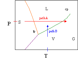
A few more points about the features of the pure component phase diagram. The regal line plant the sublimation curve, while the boiling point and melting betoken curves have already been discussed. The triple point is the unique pressure and temperature were we could have all iii phases nowadays simultaneously. At that temperature and force per unit area in our piston, we could have water ice floating in h2o, and h2o vapor above it. Once we change the temperature or pressure just a fiddling bit, nosotros can go right to a single phase. For instance, increasing the temperature by ane°C would immediately give a system of only vapor; decreasing the temperature i degree puts every molecule in a solid lattice (ice); and increasing the pressure past whatever amount places the entire system in the liquid phase.

The disquisitional point, labeled cp, is the point at which we can no longer distinguish the liquid from the gas phase, or amend said, we have a phase that is neither a gas nor a liquid, simply rather one that has properties intermediate of the ii phases. And lastly, at high temperatures, such every bit those higher that the disquisitional temperature, our vapor becomes a gas considering it is far from its condensation temperature.

Caption:

For a ii component arrangement, such as water and ethanol, we now have to take into account the corresponding mole fractions of each component in a phase diagram. We didn't have this for pure component phase diagrams because the mole fraction there is always ane because it was a pure component. Since we need take mole fractions into account here, nosotros have to accept a dissimilar arroyo to plotting the phase equilibrium for the system. Two common ways are plotting mole fractions vs. temperature (at some constant P), or plotting mole fractions vs. pressure (at some constant T), referred to as T_xy and P_xy diagrams. Here, Psub>xy diagrams are discussed thoroughly, and Tsub>xy diagrams are briefly commented on later.

Psub>xy Diagrams:

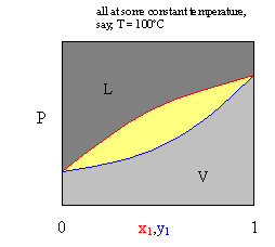
Psub>xy and Tsub>xy diagrams requite us information on vapor-liquid equilibrium. This is denoted by the enclosed yellow section on this graph. The yellow region constitutes the two phase (vapor and liquid) region. The red curve designates the bubble point curve, where the first formulation of a vapor occurs. The bluish curve designates the dew signal curve, where the first driblet of liquid condenses from a vapor. Now, consider the phase diagram beneath.

At P_i, we only have a liquid, and at P_{half dozen} we only accept a gas. Thus, for P_ane, we only take a liquid, but we don't know the mole fraction of the first component (only that the mole fraction of the gas phase is zero crusade there is no gas phase). For P₆, we tin utilize an analagous caption with cypher liquid phase.

If we were at P₁ initially, where we take a liquid mixture, and we reduce the pressure to P_ii, the first vapor molecule forms at the pressure level (and temperature) of the pure component (the pure boiling point). Similarly, P₅ is the pressure (and temperature) at which the stage change (either vaporization of the liquid or condensation of the gas) takes place.
For the equilibrium tie line at P₃, information technology is important to annotation that the upper bend (reddish) gives the liquid mole fraction of component i, x₁, and the lower curve (blue) gives the vapor mole fraction for component ane. And then, at P₃, our line shows that x₁

» .vi (interception of the bubble point bend (scarlet)), and y₁ » .8 (interception of the dew point curve (blueish)). And, of class nosotros have two components, and the second component mole fractions would just be one minus the first (ex, at point 3, x_two = .4, and y₂ = .ii). At P₄, our line shows that x_i » .45 (interception of the bubble bespeak curve (red)), and y₁ » .seven (interception of the dew point bend (blue)).

We could easily derive this stage diagram experimentally. Because nosotros are changing pressure, we could practise this by placing water and ethanol in a piston (corresponding to P₆ below). We would printing down until we encounter condensate where we could stop and take a sample of both the vapor and of the condensate in the arrangement(P5 below). Nosotros could keep to do this (giving data such as those at P_four, P_three, and P₂ below), pushing down, increasing the pressure, and sampling the vapor and condensate several times equally more vapor continues to condense until nosotros accept completely condensed the vapor. After that, increasing the pressure level would provide no further information.

If this were a binary phase diagram for a water-ethanol arrangement and we called water component one, and ethanol component ii, at P₁ we would have a liquid mixture of water and ethanol with negligible vapor higher up it. However, the diagram does tell u.s.a. the mole fractions (again, hither, there is just ane stage, a liquid phase (these are chosen two phase diagrams for a reason). The diagram gives u.s.a. concentration information merely if we are in 2 phase equilibrium, and not, for example, at P₁ or P_six. At P₂, our line at that force per unit area (necktie line) shows the vaporization (or condensation) conditions of pure water. At P_three, our line at that pressure (tie line) shows that both 10_H20 » .6 and y_Water » .8. Thus x_etOH » .iv and y_etOH » .two. And similarly, we can determine the vapor and liquid mole fractions for h2o and ethanol at P_iv. P₅ tells united states the boiling bespeak of pure ethanol, and all P₆ tells u.s.a. is that there is only a vapor phase nowadays.

T_xy Diagrams:

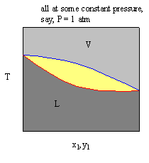
The T_xy diagram is read analogously to the P_xy diagram. The information about vapor-liquid equilibrium is given by horizontal tie lines that intersect the yellow region, as was the case with the P_xy diagrams. Experimentally, nosotros were able to obtain the P_xy diagram by slowly calculation pressure level to an all vapor water-ethanol mixture and recording the condensate composition at several dissimilar times until the vapor was completely condensed. To derive a T_xy diagram, we could simply heat a bulb of a water-ethanol liquid mixture (keeping the pressure of the arrangement constant by keeping it open to the atmosphere, P = 1 atm), and take sample of the vapor and the liquid at dissimilar temperatures, until all the liquid has been vaporized.

stinsonacess1975.blogspot.com

Source: https://uweb.engr.arizona.edu/~blowers/201project/GLsys.Diagrams.pg1.HTML

Share this post